Retrieval Augmented Generation (RAG) with Llama Index and Open-Source Models
Learn how to effectively use proprietary data with your open-source LLMs in Python
Welcome to part 4 of this AI Engineering open-source models tutorial series. Click here to view the full series.
Post Sections
Skip to section 3 if you just want code
1. What is Retrieval Augmented Generation (RAG)
2. Intro to Llama Index
3. Using Open Source Models with Llama Index - Python Code Starts Here
4. Persisting Embeddings
5. Why Open-Source RAG is a Big Deal
What is Retrieval Augmented Generation (RAG)
As I explained in my introduction to LLMs post, top LLMs like OpenAI’s GPT-4 are trained on vast amounts of data - a significant chunk of the internet is compressed. But it’s not trained on private data. So when you ask your LLM to opine about your latest slack rant, emails from your boss, or your grandma’s magic cookie recipe, even the mightiest LLM is going to struggle (and maybe hallucinate, as we’ll see).
Retrieval Augmented Generation (RAG) changes all that.
In RAG, your data is loaded and prepared for queries or “indexed”. User queries act on the index, which filters your data down to the most relevant context. This context and your query then go to the LLM along with a prompt, and the LLM provides a response. This allows you to circumvent the input token length limitations that all models have (i.e. you can’t just copy and paste your last 5 years of emails into a prompt).
You can break the Retrieval Augmented Generation process down into the following steps:
- Loading: This process involves transferring your data from its original location - which could be text files, PDFs, other websites, databases, or APIs - into your processing pipeline.
- Indexing: This step involves creating a data structure that enables you to search through the data. In language models, this typically involves creating vector embeddings (we’ll talk about these more in a minute), which are numerical representations capturing the meaning of your data.
- Storing: After indexing your data, it’s common practice to store the index and any associated metadata. This storage prevents the need for re-indexing in the future.
- Querying: Depending on the chosen indexing strategy, there are multiple ways to use language models to conduct searches. These include sub-queries, multi-step queries, and hybrid approaches.
- Evaluation: An essential phase in any pipeline is to assess its effectiveness. This can be compared to other strategies or evaluated for changes over time. Evaluation provides objective metrics on the accuracy, reliability, and speed of your query responses.
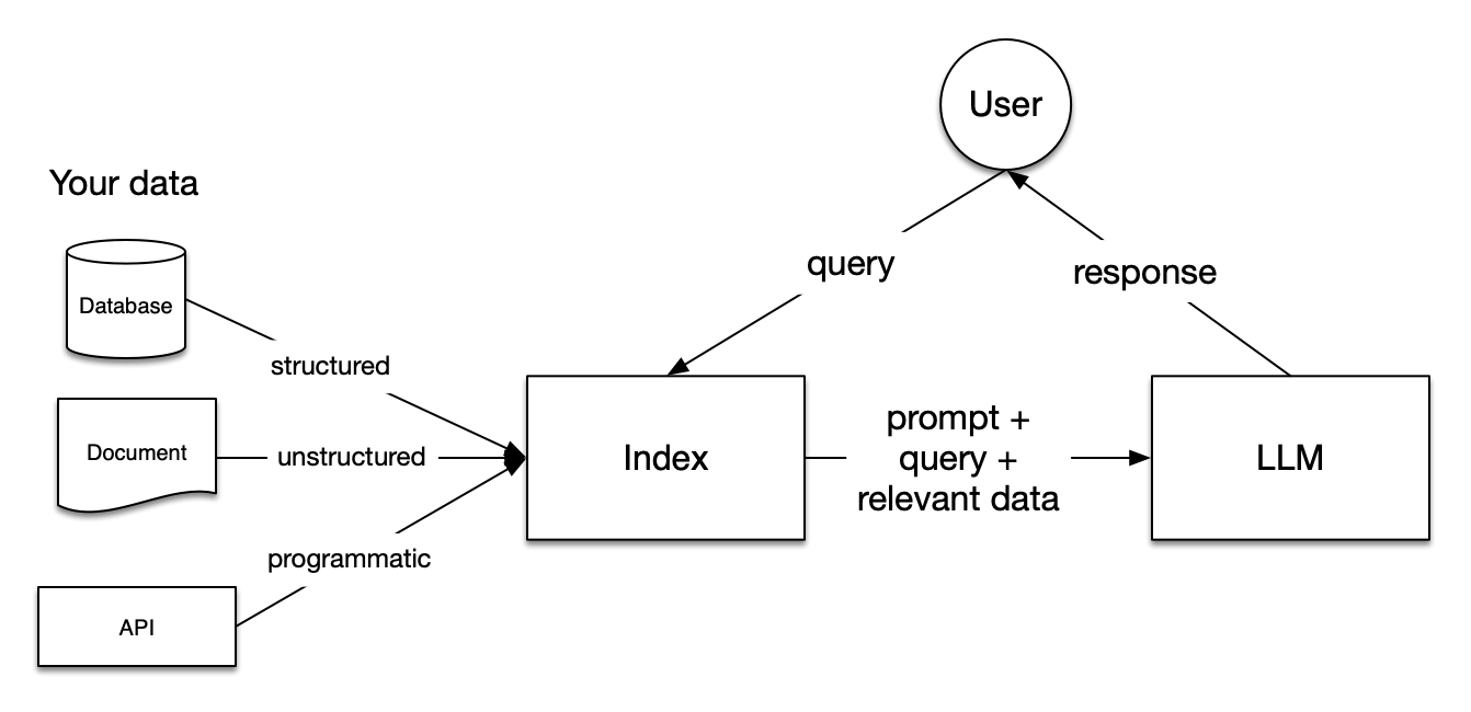
The RAG pipeline, during the querying phase, sources the most pertinent context from a user’s prompt, forwarding it along to the Large Language Model. This equips the LLM with current / private knowledge beyond its foundational training data.
RAG is basically just a really advanced form of prompt engineering.
A bunch of fancy lookups occur, some extra text snippets are sourced, and these are concatenated with (or perhaps replace) the original prompt. It’s not simple, but it’s not horrendously complicated either.
Embeddings
An important concept to understand (not just for RAG, but for ML work in general) is that of embeddings. The best article I’ve found on this is Simon Willison’s Embedding article, so I recommend checking that out. The brief summary is this:
- Embeddings are based around one trick: take a piece of content, say some text, and turn that piece of content into an array of floating point numbers.
- The key thing about that array is that it will always be the same length, no matter how long the content is. The length is defined by the embedding model you are using—an array might be 300, or 1,000, or 1,536 numbers long.
The best way to think about this array of numbers is to imagine it as co-ordinates in a very weird multi-dimensional space.
It’s hard to visualize 1,536 dimensional space, so here’s a 3D visualization of the same idea:
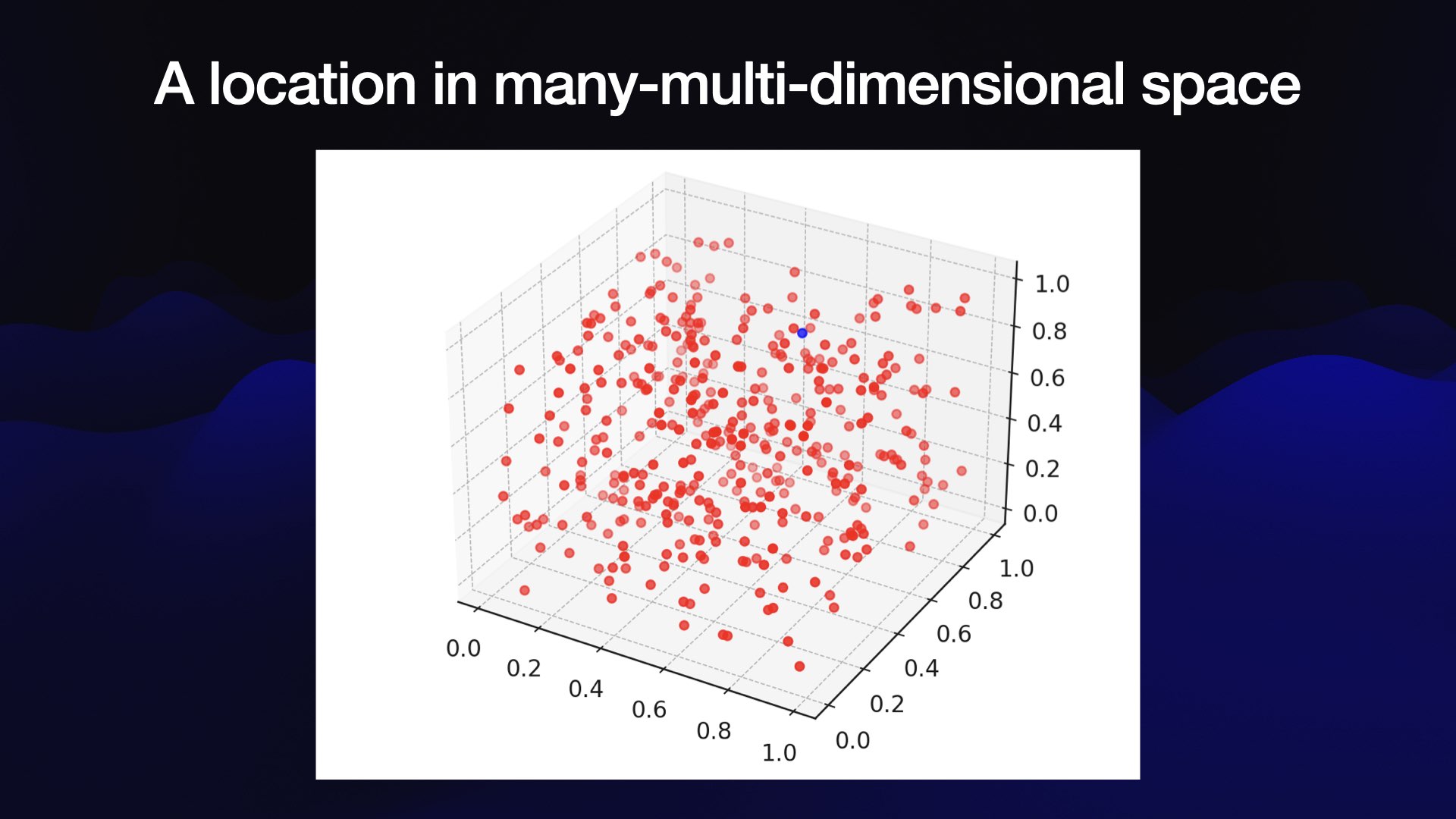 source: Simon Willison’s Blog
When you place content in this kind of multidimensional space, you can gather useful information based on the content’s position. More specifically, based on what other content is nearby.
The content location in the multidimensional space can be mathematically shown to relate to the semantic meaning of the content. This allows you to group related content based on its coordinates. Now exactly in what way the content is related depends on the model - there is potentially huge variety. Using techniques like cosine similarity or dot product allows you to build very useful functionality on different kinds of knowledge bases like:
- Search
- Recommendation systems
- Text summarization
- Image recognition
- Many more
Some important things to take note of: The array length of your embedding model is unique to that embedding model. This means that you can’t switch out one embedding model for another without having to reindex everything.
Why does this matter? Well, this is a great example of where using an open-source model gives you extra control in case a proprietary embedding model becomes unavailable. This is not unheard of:
A few months back, OpenAI announced the deprecation of several older embeddings models, as mentioned in their blog post. This presents a challenge for those who have stored extensive embeddings using these outdated models. To incorporate any new embeddings, it’s necessary to recompute the existing ones using a currently supported model.
This is a clear advantage of using an open-source model, even though proprietary embedding APIs are surprisingly cheap, and rapidly getting cheaper.
What Have Embeddings Got to Do With RAG?
Embeddings play a crucial role in the Retrieval-Augmented Generation (RAG) process, particularly in the retrieval phase. In particular:
- Vectorization of Queries and Documents: In the retrieval phase of RAG, both the user’s query (prompt) and the documents in the database are transformed into embeddings. These embeddings are high-dimensional vector representations that capture the semantic meaning of the text.
Storage and retrieval of these embeddings has led to a boom in vector database technologies, which we’ll discuss later in this post.
Embeddings in RAG are used to bridge the gap between the user’s query and the relevant information contained in a large corpus of documents. They enable the system to understand and match the semantic content of the query with relevant documents, which is a key step in generating informative and contextually relevant responses.
RAG vs. Fine Tuning
As the creator of LlamaIndex (which we’ll look at in the next section) Jerry Liu says:
RAG is just a hack
but RAG is a very powerful hack! It can radically transform the performance of your LLM.
Users will immediately bump up against the limits of generative AI anytime there’s a question that requires information that sits outside the LLM’s training corpus, resulting in hallucinations, inaccuracies, or deflection. Both RAG and finetuning are solutions to this problem, there are differences:
- RAG is easier: RAG requires less complex AI knowledge. As Quentin Anthony from Eleuther notes “the Math for finetuning isn’t well known yet”. Furthermore, finetuning requires GPU time, which can be costly and slow. In contrast, RAG is basically just data engineering once you learn the tools.
- Stricter access control and higher visibility: when finetuning, the model learns everything. With RAG, you can decide what documents the index should have access to, making it more secure by default. You also have much better interpretability and observability metrics as you can look at the context if a response doesn’t seem right.
- Context window limitation: you can only fit so many tokens into the prompt due to the way models work. Finetuning helps you circumvent that by compressing the knowledge into the model weights rather than putting it in the prompt. Because more and more open source models have 100k+ token context windows, this limitation is rapidly becoming less of an issue.
Introduction to LlamaIndex
LlamaIndex has crossed 600,000 monthly downloads, raised $8.5M from Greylock, and has a fast growing open source community that contributes to LlamaHub.
LlamaHub made it easy for developers to import data from Google Drive, Discord, Slack, databases, and more into their LlamaIndex projects. Along with LangChain LlamaIndex is one of the most popular tools for AI engineers. I think the learning curve on LangChain can be a bit steep, and that some of the abstractions they have chosen render the library unnecessarily unreadable. LlamaIndex, on the other hand, is very intuitive.
Using Open Source Models with Llama Index - Code Starts Here
If you haven’t already read the post on using open-source models with Llama.cpp, be sure to check that out so you have the necessary foundation.
Setup
- Create your virtualenv / poetry env
pip install llama-index transformers
To begin, we instantiate our open-source LLM. Once again we’ll be using the GGUF model format:
from llama_index.llms import LlamaCPP
from llama_index.embeddings import HuggingFaceEmbedding

llm = LlamaCPP(
    model_path="path/to/your/model/Mixtral_8x7B_Instruct_v0.1.gguf",  # https://huggingface.co/TheBloke/Mixtral-8x7B-Instruct-v0.1-GGUF
    context_window=32000,
    max_new_tokens=1024,
    model_kwargs={'n_gpu_layers': 1},
    verbose=True
)

embedding_model = HuggingFaceEmbedding(model_name="WhereIsAI/UAE-Large-V1")  # https://huggingface.co/WhereIsAI/UAE-Large-V1
An important gotcha is that you need to use the llama_index LlamaCPP class. You can’t use the llama_cpp Llama class (easy mistake to make).
Notice in the above code snippet that I’m instantiating a separate model for the embeddings. This is because a dedicated embedding model is much better suited to that task.
Tokenization
By default, LlamaIndex uses a global tokenizer for all token counting. This defaults to cl100k from tiktoken.
If you change the LLM like we have done, you may need to update this tokenizer to ensure accurate token counts, chunking, and prompting.
Luckily, this is quite straight-forward with the transformers library:
from transformers import AutoTokenizer
from llama_index import set_global_tokenizer

set_global_tokenizer(
    AutoTokenizer.from_pretrained("mistralai/Mixtral-8x7B-Instruct-v0.1").encode  # pass in the HuggingFace model org + repo
)
Now that we’ve got our models and set the global tokenizer, we are ready to setup the LlamaIndex ServiceContext:
The ServiceContext is a bundle of commonly used resources used during the indexing and querying stage in a LlamaIndex pipeline/application. You can use it to set the global configuration, as well as local configurations at specific parts of the pipeline.
from llama_index import ServiceContext

service_context = ServiceContext.from_defaults(
    llm=llm,
    embed_model=embedding_model,
    system_prompt='You are a bot that answers questions about podcast transcripts'
)
Crucially, we have overriden the defaults (which uses OpenAI’s gpt-3.5-turbo) to use our open-source LLM and embedding model. Now we can proceed with creating our index. In this case, we’re going embed the transcript for episode 44 of the Latent Space podcast, which you should check out.
Before your chosen LLM can act on your data, you first need to process the data and load it. This has parallels to data cleaning/feature engineering pipelines in the ML world, or ETL pipelines in a traditional data engineering setting.
from pathib import Path
import glob
from llama_index import SimpleDirectoryReader, VectorStoreIndex

# Find all files that match the pattern "*transcript*" using the Python standard library glob module
transcript_files = glob.glob(str(Path(transcript_directory) / '**/*transcript*'), recursive=True)

documents = SimpleDirectoryReader(input_files=transcript_files).load_data()

# We pass in the service context we instantiated earlier (powered by our open-source LLM)
index = VectorStoreIndex.from_documents(documents, service_context=service_context, show_progress=True)
What the above code does is (1) Reading the documents (in this case our transcript JSON file) using the
SimpleDirectoryReader
SimpleDirectoryReader is the simplest way to load data from local files into LlamaIndex. For production use cases it’s more likely that you’ll want to use one of the many Readers available on LlamaHub, but SimpleDirectoryReader is a great way to get started.
LlamaIndex has the notion of Data Connectors aka Readers to ingest data from different sources and in different formats. You can browse
these on LlamaHub.
Then we create a VectorStoreIndex:
Vector Stores are a key component of retrieval-augmented generation (RAG) and so you will end up using them in nearly every application you make using LlamaIndex, either directly or indirectly.
Great! We now have an index which includes our transcript. The last thing we need to do is setup our prompt and query:
query_engine = index.as_query_engine()
result = query_engine.query("According to Dylan Patel, what don't people understand about the semiconductor supply chain?")
I setup a script to query the LlamaCPP LLM (i.e. without using RAG) and it gave me this response:
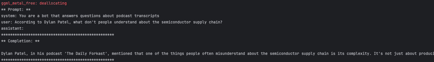
This is interesting! Mixtral-8x7b is a really powerful LLM, and gives quite a reasonable sounding response:
Dylan Patel, in his podcast ‘The Daily Forkast’, mentioned that one of the things people often misunderstand about the semiconductor supply chain is its complexity. It’s not just about producing a chip and then shipping it; there are multiple stages involved, including design, manufacturing, testing, packaging, and logistics. Each stage has its own set of challenges and dependencies, making the entire process quite intricate…[continues]
However, Mixtral has hallucinated. Dylan Patel doesn’t have a podcast called “The Daily Forecast”. Nor does this answer capture the nuance of his real opinion.
Here’s the result from our RAG enabled model:
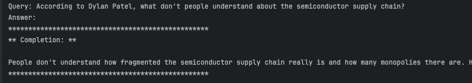
People don’t understand how fragmented the semiconductor supply chain really is and how many monopolies there are. He emphasizes that it involves numerous specific technologies requiring various companies with high market shares, which are often overlooked or considered inconsequential due to their smaller revenue size… [Continues]
This answer captures exactly what Dylan said in episode 44 of the Latent Space podcast.
Our LLM just became more powerful.
Debugging
Here are a few quick debugging tips:
Basic logging The simplest possible way to look into what your application is doing is to turn on debug logging.
LlamaIndex provides callbacks to help debug, track, and trace the inner workings of the library. Using the callback manager, as many callbacks as needed can be added. In addition to logging data related to events, you can also track the duration and number of occurrences of each event.
For example, the LlamaDebugHandler will, by default, print the trace of events after most operations.
You can enable debug logging and get a simple callback handler like this:
import logging
import sys
import llama_index

logging.basicConfig(stream=sys.stdout, level=logging.DEBUG)
logging.getLogger().addHandler(logging.StreamHandler(stream=sys.stdout))
llama_index.set_global_handler("simple")
Persisting
By default, the VectorStoreIndex stores everything in memory. The most basic form of persistence (for playing around on our local dev environment)
is to just use flat file storage. You can do this like so:
import glob
import logging
from pathlib import Path

from llama_index import ServiceContext, StorageContext, \
    load_index_from_storage, SimpleDirectoryReader, VectorStoreIndex


def save_or_load_index(index_dir: Path, service_context: ServiceContext) -> VectorStoreIndex:
    index_exists = any(item for item in Path(index_dir).iterdir() if item.name != '.gitkeep')  # Checks if the directory is not empty

    if index_exists:
        logging.info(f"Loading persisted index from: {index_dir}")
        storage_context = StorageContext.from_defaults(persist_dir=index_dir)
        index = load_index_from_storage(storage_context, service_context=service_context)
    else:
        logging.info("Persisted index not found, creating a new index...")

        # Find all files that match the pattern "*transcript*"
        transcript_files = glob.glob(str(DATA_DIR / '**/*transcript*'), recursive=True)

        documents = SimpleDirectoryReader(input_files=transcript_files).load_data()
        index = VectorStoreIndex.from_documents(documents, service_context=service_context, show_progress=True)
        index.storage_context.persist(persist_dir=index_dir)

    return index
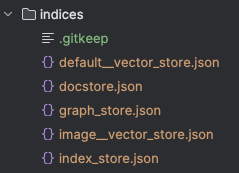
After running this code, you’ll see the vectors saved into these JSON files:
Using a Vector Database
For any serious use cases, we will rapidly outgrow flat files. This is where vector databases come in. There are hundreds of AI startups scrambling at the moment to make the best vector database in order to provide the fastest data retrieval capabilities. LlamaIndex offers many Vector Store Integrations, with some useful comparisons in their docs.
Noteworthy players include Pinecone, Chroma and Faiss. Here’s a table summarizing their merits:
| Vector Database | Homepage | Strengths | Weaknesses |
|---|---|---|---|
| Pinecone | Pinecone | Managed service, real-time data ingestion, low-latency search, scalability, integration with LangChain. | Not open-source, may have limitations for custom infrastructure setups. |
| Chroma | Chroma | Open-source, suitable for LLM applications, supports multiple data types and formats, flexible deployment options. | Newer in the market, might have fewer integrations compared to more established databases. |
| Weaviate | Weaviate | Open-source, scalable, fast searches, AI-driven search functionalities, supports large-scale deployments. | Requires more management for self-hosting compared to managed solutions. |
| Qdrant | Qdrant | Open-source, flexible API, high speed and accuracy, advanced filtering, scalability, efficient resource usage. | Being open-source, it might require more setup and maintenance effort. |
| Faiss | Faiss | Efficient for large datasets, supports various distances, batch processing, GPU integration. | As a library, it requires integration into an existing system, which might be complex for non-experts. |
I’m a PostgreSQL guy, and believe strongly in innovation tokens. So I’ll be using the postgres extension pgvector since that means I don’t have to add an entirely new database system to my stack. Also, my favorite PaaS Render supports pgvector.
Once you’ve installed the pgvector extension, here’s how we can create the index (and persist the embeddings) in postgreSQL:
from llama_index import SimpleDirectoryReader, StorageContext
from llama_index.indices.vector_store import VectorStoreIndex
from llama_index.vector_stores import PGVectorStore
import textwrap
from sqlalchemy import make_url

import psycopg2

connection_string = "postgresql://postgres:password@localhost:5432"
db_name = "vector_db"
conn = psycopg2.connect(connection_string)
conn.autocommit = True

with conn.cursor() as c:
    c.execute(f"DROP DATABASE IF EXISTS {db_name}")
    c.execute(f"CREATE DATABASE {db_name}")


url = make_url(connection_string)
vector_store = PGVectorStore.from_params(
    database=db_name,
    host=url.host,
    password=url.password,
    port=url.port,
    user=url.username,
    table_name="transcripts",
    embed_dim=1024,  # WhereIsAI/UAE-Large-V1 embedding dimension
)

storage_context = StorageContext.from_defaults(vector_store=vector_store)
index = VectorStoreIndex.from_documents(
    documents, storage_context=storage_context, show_progress=True
)
query_engine = index.as_query_engine()

response = query_engine.query("Who is Dylan Patel?")

print(textwrap.fill(str(response), 100))
Something important to note here is that you need to figure out the number of dimensions of your
embedding model. In this post we used the WhereIsAI/UAE-Large-V1 embedding model. I couldn’t find the n_dimensions for this model
documented on huggingface or github (welcome to the challenges of Open-Source), so I just ran:
embedding_model._embed(['yo', 'yoyo']) and looked at the result length, which told me the n_dimensions was 1024. If you are using
a different embedding model, you will need to update this value.
There is also a helpful library for working with pgvector in python.
Update: I’ve now written a detailed post on how to work with postgres.
Why Open-Source RAG is a Big Deal
Applications of RAG
There are a lot of well known applications of RAG like:
- Question Answering: RAG can provide detailed, accurate answers by retrieving relevant information before generating a response.
- Content Creation: In tasks like article writing, RAG can pull in relevant facts and figures, enriching the content.
- Dialogue Systems: It can enhance chatbots by providing them with a wealth of information, making conversations more informative and engaging.
We can classify these Data-backed Large Language Model (LLM) applications into three main types:
-
Query Engines: These are end-to-end pipelines that process natural language queries and return responses with relevant context, enabling users to ask questions over their data.
-
Chat Engines: Chat engines facilitate back-and-forth conversations with data, unlike the single question-and-answer format of query engines.
-
Agents: Agents are automated decision-makers powered by LLMs. They interact with the world through various tools, taking multiple steps and dynamically choosing actions to complete tasks, offering flexibility for complex tasks.
When you mix and match these types of applications with open-source LLMs and RAG I get particularly excited.
When people are able to use LLMs on their own private data without relying on dubious (and leaky!) corporations, then you will start to see:
- The ability to make text/voice notes on your phone that are automatically categorized and generate mind maps and connections with other related notes.
- The ability to play back conversations on your phone and receive coaching on your latest sales call approach on device
- The ability to perform really detailed and meaningful health studies based on personal health data on device
And that’s just the tip of the iceberg. I really wouldn’t want to be competing against someone fully leveraging this tech for their second brain in 5 years time.